Lidar Scan API

In this reference document, we explain a core concept in both C++ and Python, and will often link function names in the order (C++ class/function, Python class/function). For language-specific usage and running example code, please see the Python LidarScan examples or the C++ LidarScan examples.

The LidarScan class (ouster::LidarScan, LidarScan) batches lidar packets by full rotations into accessible fields of the appropriate type. The LidarScan also allows for easy projection of the batched data into Cartesian coordinates, producing point clouds.

Creating the LidarScan

A LidarScan (ouster::LidarScan, LidarScan) contains fields of data specified at its initialization either through a lidar profile or a specific list of fields:

scan = LidarScan(h, w, info.format.udp_profile_lidar)

auto profile_scan = ouster::LidarScan(w, h, info.format.udp_profile_lidar);

Since each LidarScan corresponds to a single frame (and is batched accordingly), you can access the frame_id with simply:

frame_id = scan.frame_id # frame_id is an int

int32_t frame_id = scan.frame_id

In addition to frame_id and the fields specified at initialization, a LidarScan also contains the column header information: timestamp, status, measurement_id. These are aggregated from each measurement block into W-element arrays, which are represented as an Eigen::Array and a numpy.ndarray in C++ and Python respectively. Note that if you use set the sensor configuration parameter azimuth_window to something less than the full width, the values in the header outside the azimuth window will be 0’d out accordingly.

# each of these has as many entries as there are columns in the scan
ts_0 = scan.timestamp[0]
measurement_id_0 = scan.measurement_id[0]
status_0 = status[0]

auto ts = profile_scan.timestamp();
auto status = profile_scan.status();
auto measurement_id = profile_scan.measurement_id();

For any field contained by a LidarScan scan, you can access that field in the following way:

ranges = scan.field(client.ChanField.RANGE)
ranges2 = scan.field(client.ChanField.RANGE2)
reflectivity = scan.field(client.ChanField.REFLECTIVITY)
reflectivity2 = scan.field(client.ChanField.REFLECTIVITY2)

auto range = profile_scan.field<uint32_t>(ChanField::RANGE);

Finally, the fields of an existing LidarScan can be found by accessing the fields of the scan through an iterator:

scan = next(scans)
print("Available fields and corresponding dtype in LidarScan")
for field in scan.fields:
    print('{0:15} {1}'.format(str(field), scan.field(field).dtype))

for (const auto& kv : scan.fields()) {
    auto field_name = kv.first;
    // auto& field = kv.second;
    std::cerr << "\t" << field_name << "\n ";
}

Note

The units of a particular field from a LidarScan are consistent even when you use lidar profiles which scale the returned data from the sensor. This is because the LidarScan will reverse the scaling for you when parsing. For example, the RANGE field on a LidarScan constructed with the low data rate profile will be in millimeters even though the return from the sensor is given in 8mm increments.

Running the above code on a sample LidarScan will give you output that looks like:

Available fields and corresponding dtype in LidarScan
RANGE           uint32
RANGE2          uint32
SIGNAL          uint16
SIGNAL2         uint16
REFLECTIVITY    uint8
REFLECTIVITY2   uint8
NEAR_IR         uint16

Now that we know how to create the LidarScan and access its contents, let’s see what we can do with it!

Adding custom fields to a LidarScan

Beginning in Ouster SDK 0.12.0, it’s possible to add custom fields to a LidarScan. This is especially useful if you want to add custom data to an OSF file for visualization purposes. Like the standard fields normally found in a LidarScan, custom fields also make use of Eigen::Array and numpy.ndarray in C++ and Python, respectively.

lidar_scan = client.LidarScan(128, 1024)
lidar_scan.add_field("my-custom-field", np.uint8, ())
lidar_scan.field("my-custom-field")[:] = 1  # set all pixels
lidar_scan.field("my-custom-field")[10:20, 10:20] = 255  # set a block of pixels

auto custom_scan = ouster::LidarScan(info);
custom_scan.add_field("my-custom-field",
                      ouster::fd_array<uint8_t>(info.h(), info.w()));

// Custom fields
custom_scan.field<uint8_t>("my-custom-field") = 1;  // set all pixels
custom_scan.field<uint8_t>("my-custom-field").block(10, 10, 20, 20) =
    255;  // set a block of pixels

Note - fields can also be removed using the del_field method. This can be useful for removing unneeded data, thereby saving space when saving scans to an OSF file.

Projecting into Cartesian Coordinates

To facilitate working with 3D points, you can create a pre-computed XYZ look-up table XYZLut (ouster::XYZLut, client.XYZLut()) on the appropriate metadata, which you can then use to project the RANGE and RANGE2 fields into Cartesian coordinates efficiently. The result of calling this function will be a point cloud represented as an array (either an Eigen::Array or a numpy array). See the respective API documentations for ouster::cartesian() and client.XYZLut() for more details.

# transform data to 3d points
xyzlut = client.XYZLut(metadata)
xyz = xyzlut(scan.field(client.ChanField.RANGE))

XYZLut lut = make_xyz_lut(info, true);
auto range = scan.field(sensor::ChanField::RANGE);
auto cloud = cartesian(range, lut);

Once you have your x, y, and z values, you can plot them easily to get something like:

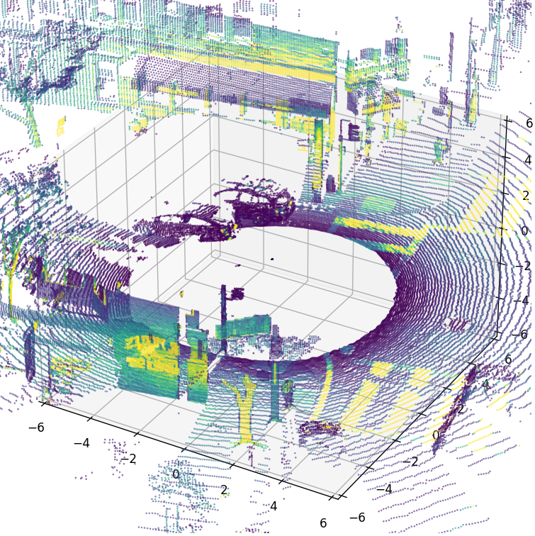
../_images/lidar_scan_xyz_84.png — Point cloud from OS1 sample data (scan 84). Points colored by `SIGNAL` value.

To see how to generate this image, see the Python LidarScan examples.

Staggering and Destaggering

The default representation of LidarScan stores data in staggered columns, meaning that each column contains measurements taken at a single timestamp. As the lasers flashing at each timestamp are arranged over several different azimuths, the resulting 2D image if directly visualized is not a natural image.

Let’s take a look at a typical staggered representation:

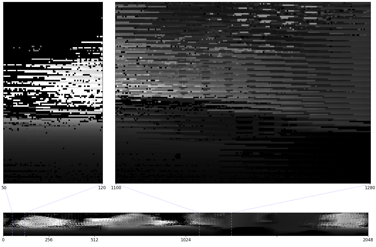
../_images/lidar_scan_staggered.png — LidarScan `RANGE` field visualized with `matplotlib.pyplot.imshow()` and simple gray color mapping for better look.

It would be convenient to obtain a representation where the columns represent azimuth angle instead of timestamp. For this natural 2D image, we destagger the relevant field of the LidarScan with destagger (ouster::destagger(), client.destagger() function):

ranges = scan.field(client.ChanField.REFLECTIVITY)
ranges_destaggered = client.destagger(source.metadata, range)

auto reflectivity_destaggered =
    destagger<uint32_t>(reflectivity, info.format.pixel_shift_by_row);

The above code gives the scene below (see the long strip at the bottom). We’ve magnified two patches for better visibility atop.

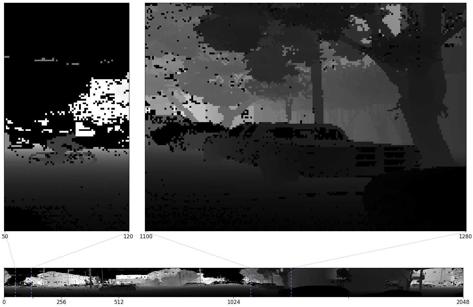
../_images/lidar_scan_destaggered.png — **destaggered** LidarScan `RANGE` field

After destaggering, we can see the scene contains a man on a bicycle, a few cars, and many trees. This image now makes visual sense, and we can easily use this data in common visual task pipelines.

Populating LidarScans

This reference has covered how to a LidarScan, and how to access, project, and destagger its contents. But in order for LidarScan s to be useful, we need a way to populate them with packet data! For convenience, the Ouster Python SDK provides the Scans interface, which allows both sampling, used in Visualization with Matplotlib, and streaming, used in Streaming Live Data.

Under the hood, this class batches packets into LidarScans. C++ users must batch packets themselves using the ouster::ScanBatcher class. To get a feel for how to use it, we recommend reading this example on GitHub.