PointViz Tutorial & API Usage

Environment and General Setup

In this interactive tutorial we explore the Python bindings of the viz.PointViz and how we can use it programmatically to visualize various 2D and 3D scenes.

Note

We assume you have downloaded the sample data and set SAMPLE_DATA_PCAP_PATH and SAMPLE_DATA_JSON_PATH to the locations of the OS1 128 sample data pcap and json files correspondingly.

Before proceeding, be sure to install ouster-sdk Python package, see OusterSDK Python Installation for details.

This interactive tutorial will open a series of visualizer windows on your screen. Each example can be exited by pressing ESC or the exit button on the window; doing so will open the next visualizer window.

Let’s start the tutorial:

python3 -m ouster.sdk.examples.viz $SAMPLE_DATA_PCAP_PATH $SAMPLE_DATA_JSON_PATH

Now you can proceed through each example, labeled by numbers to match your screen output.

Creating an empty PointViz window

viz.PointViz is the main entry point to the Ouster visualizer, and it keeps track of the window state, runs the main visualizations loop, and handles mouse and keyboard events.

To create the PointViz window (and see a black screen as nothing has been added), you can try the following:

# Creating a point viz instance
point_viz = viz.PointViz("Example Viz")
viz.add_default_controls(point_viz)

# ... add objects here

# update internal objects buffers and run visualizer
point_viz.update()
point_viz.run()

As expected we see a black empty window:

Empty PointViz window

Now let’s try to add some visual objects to the viz. Hit ESC or click the exit button on the window to move to the next example.

Images and Labels

Some of the basic 2D objects we can add include the 2D viz.Label and the viz.Image. To add these, we need an understanding of the 2D Coordinate System for viz.PointViz.

The Image object

To create a 2D Image you need to use the viz.Image object. Currently only normalized grayscale images are supported, though you can use viz.Image.set_mask(), which accepts RGBA masks, to get color.

The viz.Image screen coordinate system is height-normalized and goes from bottom to top ([-1, +1]) for the y coordinate, and from left to right ([-aspect, +aspect]) for the x coordinate, where:

aspect = viewport width in Pixels / viewport height in Pixels

Here is how we create a square image and place it in the center:

img = viz.Image()
img.set_image(np.full((10, 10), 0.5))
img.set_position(-0.5, 0.5, -0.5, 0.5)
point_viz.add(img)

Expected result: (without top and bottom labels)

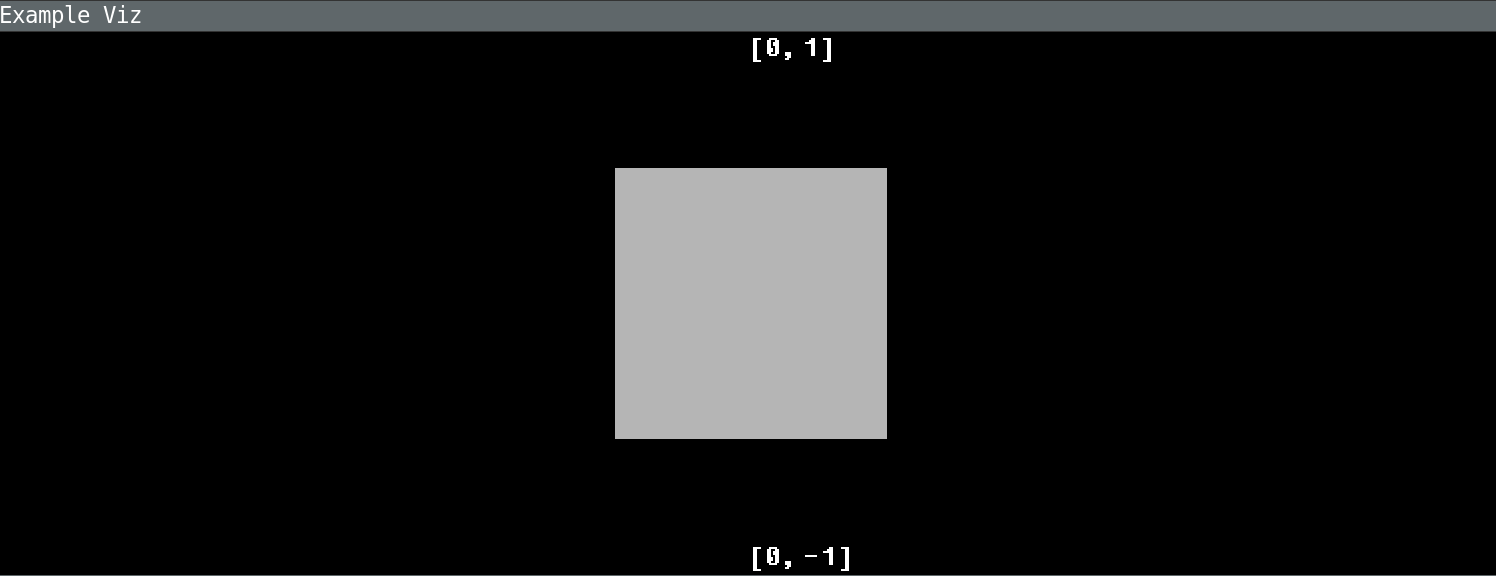
viz.Image.set_position() to center image

Window-aligned Images

To align an image to the left or right screen edge, use viz.Image.set_hshift(), which accepts a width-normalized ([-1, 1]) horizontal shift which is applied to the image position after the viz.Image.set_position() values are first applied.

Here is how we place an image to the left edge of the screen:

# move img to the left
img.set_position(0, 1, -0.5, 0.5)
img.set_hshift(-1)

Expected result:

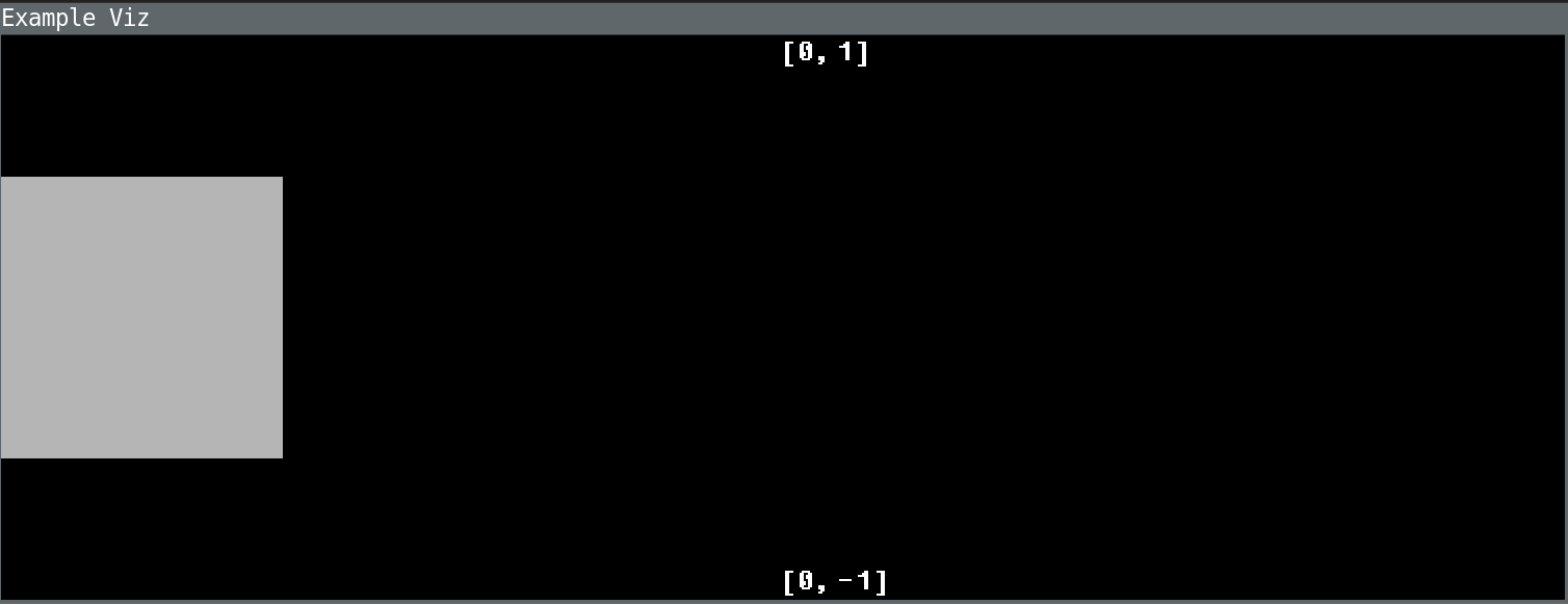
viz.Image.set_position() with viz.Image.set_hshift() to align image to the left

And here’s how we place an image to the right edge of the screen:

# move img to the right
img.set_position(-1, 0, -0.5, 0.5)
img.set_hshift(1)

Expected result:

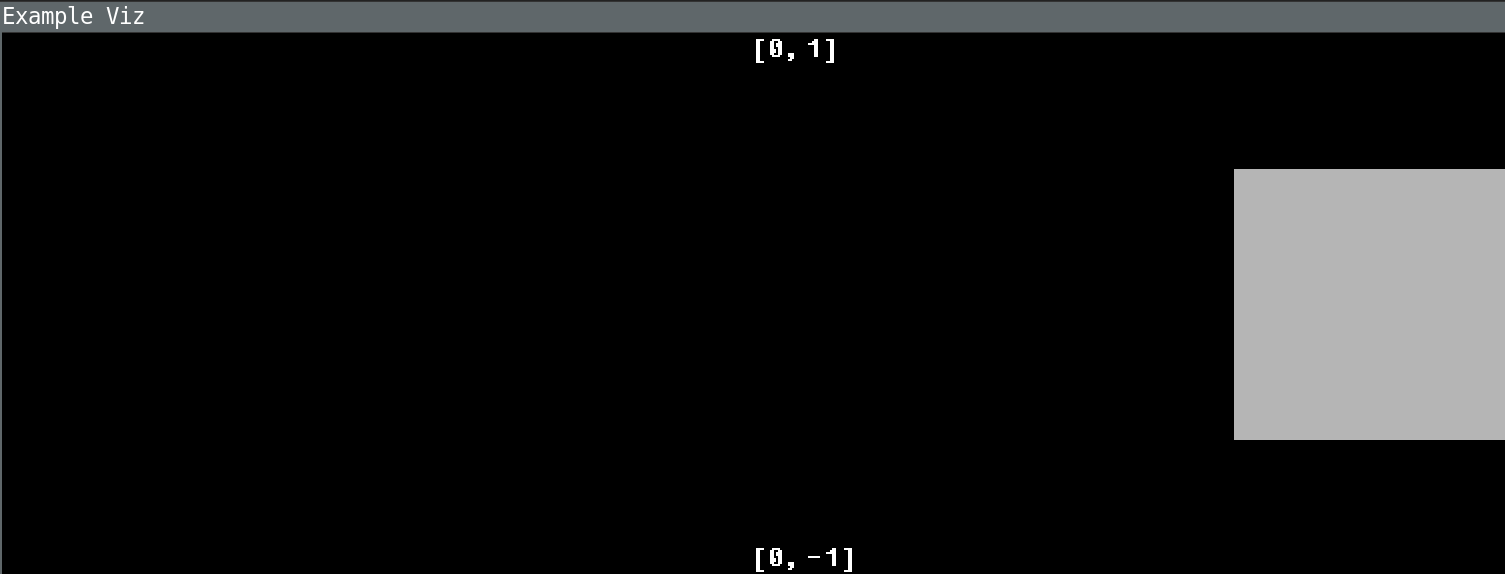
viz.Image.set_position() to align image to the right

Finally, here’s how we place an image to the right edge and bottom of the screen:

# move img to the right bottom
img.set_position(-1, 0, -1, 0)
img.set_hshift(1)

Expected result:

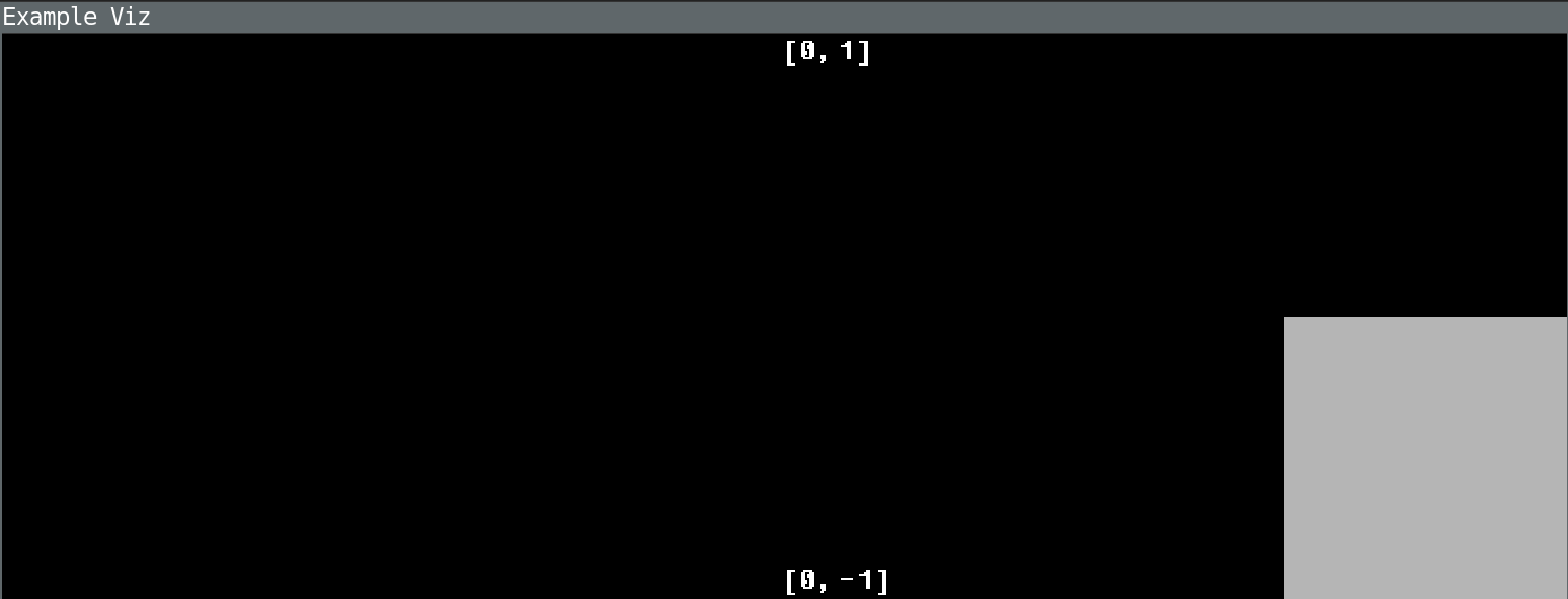
viz.Image.set_position() to align image to the bottom and right

Cool! Let’s move on to more sophisticated images!

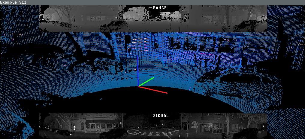
LidarScan Fields as Images

Now we can use viz.Image to visualize LidarScan fields data as images. In this example we show the RANGE and SIGNAL fields images positioned on the top and bottom of the screen correspondingly.

Note

If you aren’t familiar with the LidarScan, please see Lidar Scan API. A single scan contains a full frame of lidar data.

So how do we do it?

scan = next(scans)

img_aspect = (meta.beam_altitude_angles[0] -
              meta.beam_altitude_angles[-1]) / 360.0
img_screen_height = 0.4  # [0..2]
img_screen_len = img_screen_height / img_aspect

# prepare field data
ranges = scan.field(client.ChanField.RANGE)
ranges = client.destagger(meta, ranges)
ranges = np.divide(ranges, np.amax(ranges), dtype=np.float32)

signal = scan.field(client.ChanField.REFLECTIVITY)
signal = client.destagger(meta, signal)
signal = np.divide(signal, np.amax(signal), dtype=np.float32)

# creating Image viz elements
range_img = viz.Image()
range_img.set_image(ranges)
# top center position
range_img.set_position(-img_screen_len / 2, img_screen_len / 2,
                       1 - img_screen_height, 1)
point_viz.add(range_img)

signal_img = viz.Image()
signal_img.set_image(signal)
img_aspect = (meta.beam_altitude_angles[0] -
              meta.beam_altitude_angles[-1]) / 360.0
img_screen_height = 0.4  # [0..2]
img_screen_len = img_screen_height / img_aspect
# bottom center position
signal_img.set_position(-img_screen_len / 2, img_screen_len / 2, -1,
                        -1 + img_screen_height)
point_viz.add(signal_img)

In the highlighted lines, you can see that we’re simply using viz.Image(), viz.set_image(), and viz.set_position() like we did before, but this time with more interesting data!

Expected result:

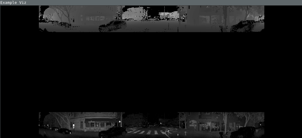
LidarScan fields RANGE and SIGNAL visualized with viz.Image

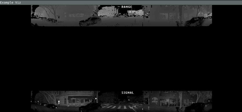
2D Label object

2D labels are represented with viz.Label object and use a slightly different coordinate system that goes from left to right [0, 1] for the x coordinate, and from top to bottom [0, 1] the for y coordinate.

Let’s apply the labels to our already visualized LidarScan field images:

range_label = viz.Label(str(client.ChanField.RANGE),
                        0.5,
                        0,
                        align_top=True)
range_label.set_scale(1)
point_viz.add(range_label)

signal_label = viz.Label(str(client.ChanField.REFLECTIVITY),
                         0.5,
                         1 - img_screen_height / 2,
                         align_top=True)
signal_label.set_scale(1)
point_viz.add(signal_label)

Expected result:

LidarScan fields images captioned with 2D viz.Label

Note

Currently the viz.Image has a different 2D coordinate system than the viz.Label. This is likely to change in the future.

Point Clouds: the Cloud object

Point Cloud visualization implemented via the viz.Cloud object can be used in two ways:

• Structured Point Clouds, where 3D points are defined with 2D field images (i.e. LidarScan fields images)

• Unstructured Point Clouds, where 3D points are defined directly as a set of XYZ 3D points

Let’s take a closer look at each of these.

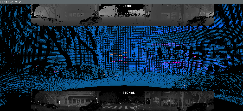
Structured Point Cloud

The Ouster sensor produces a structured point cloud as a 2D range image which can be projected into 3D Cartesian coordinates with a pre-generated lookup table. For this reason the internal implementation of viz.Cloud applies the lookup table transform automatically generated from client.SensorInfo (metadata object) and 2D RANGE image as an input.

Note

Please refer to Lidar Scan API for details about internal LidarScan representations and its basic operations.

To visualize client.LidarScan object we use the following code:

cloud_scan = viz.Cloud(meta)
cloud_scan.set_range(scan.field(client.ChanField.RANGE))
cloud_scan.set_key(signal)
point_viz.add(cloud_scan)

Expected result:

LidarScan Point Cloud with viz.Cloud as structured

Unstructured Point Clouds

Point Clouds that are represented as a set of XYZ 3D points are called unstructured for our purposes.

It’s possible to set the viz.Cloud object by setting the 3D points directly, which is useful when you have unstructured point clouds.

# transform scan data to 3d points
xyzlut = client.XYZLut(meta)
xyz = xyzlut(scan.field(client.ChanField.RANGE))

cloud_xyz = viz.Cloud(xyz.shape[0] * xyz.shape[1])
cloud_xyz.set_xyz(np.reshape(xyz, (-1, 3)))
cloud_xyz.set_key(signal.ravel())
point_viz.add(cloud_xyz)

You should see the same visualization as for the structured point clouds.

Example: 3D Axes Helper as Unstructured Points

The viz.Cloud object also supports color RGBA masks. Below is an example how we can use unstructured point clouds to draw 3D axes at the origin:

# basis vectors
x_ = np.array([1, 0, 0]).reshape((-1, 1))
y_ = np.array([0, 1, 0]).reshape((-1, 1))
z_ = np.array([0, 0, 1]).reshape((-1, 1))

axis_n = 100
line = np.linspace(0, 1, axis_n).reshape((1, -1))

# basis vector to point cloud
axis_points = np.hstack((x_ @ line, y_ @ line, z_ @ line)).transpose()

# colors for basis vectors
axis_color_mask = np.vstack((np.full(
    (axis_n, 4), [1, 0.1, 0.1, 1]), np.full((axis_n, 4), [0.1, 1, 0.1, 1]),
                             np.full((axis_n, 4), [0.1, 0.1, 1, 1])))

cloud_axis = viz.Cloud(axis_points.shape[0])
cloud_axis.set_xyz(axis_points)
cloud_axis.set_key(np.full(axis_points.shape[0], 0.5))
cloud_axis.set_mask(axis_color_mask)
cloud_axis.set_point_size(3)
point_viz.add(cloud_axis)

Expected result:

3D Axes Helper with viz.Cloud unstructured and color RGBA masks

LidarScanViz for point cloud with fields images

To make it even more easier to explore the data of client.LidarScan objects, we provide a higher-order visual component viz.LidarScanViz that enables:

• 3D point cloud and two 2D fields images in one view

• color palettes for 3D point cloud coloration

• point cloud point size increase/decrease

• toggles for view of different fields images and increasing/decreasing their size

• dual return point clouds and fields images support

• key handlers for all of the above

The majority of keyboard operations that you can see in simple-viz keymaps implemented by viz.LidarScanViz.

Let’s look at how we can explore a client.LidarScan object with a couple of lines:

# Creating LidarScan visualizer (3D point cloud + field images on top)
ls_viz = viz.LidarScanViz([meta], point_viz)

# adding scan to the lidar scan viz
ls_viz.update([scan])

# refresh viz data
ls_viz.draw()

# visualize
# update() is not needed for LidatScanViz because it's doing it internally
point_viz.run()

Not a lot of lines of code needed to visualize all the information desired!

Expected result:

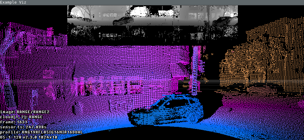
LidarScan Point Cloud with viz.LidarScanViz

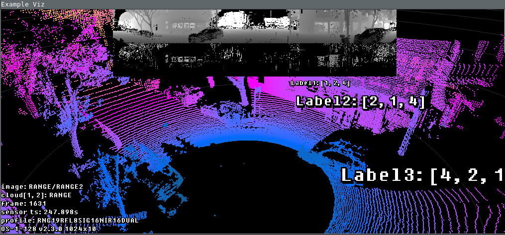
3D Label object

The same viz.Label object that we used for 2D labels can be used for putting text labels in 3D space.

Here’s an example of using 3D Labels:

# Adding 3D Labels
label1 = viz.Label("Label1: [1, 2, 4]", 1, 2, 4)
point_viz.add(label1)

label2 = viz.Label("Label2: [2, 1, 4]", 2, 1, 4)
label2.set_scale(2)
point_viz.add(label2)

label3 = viz.Label("Label3: [4, 2, 1]", 4, 2, 1)
label3.set_scale(3)
point_viz.add(label3)

Expected result:

3D viz.Label superimposed onto LidarScanViz

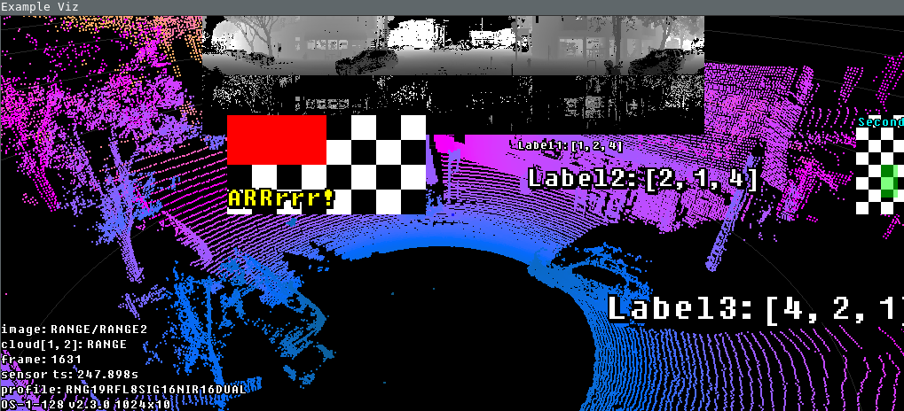
Example: Overlay 2D Images and 2D Labels

Here’s another example to show how one could add 2D Images, RGBA masks and 2D Labels added to viz.LidarScanViz:

# Adding image 1 with aspect ratio preserved
img = viz.Image()
img_data = make_checker_board(10, (2, 4))
mask_data = np.zeros((30, 30, 4))
mask_data[:15, :15] = np.array([1, 0, 0, 1])
img.set_mask(mask_data)
img.set_image(img_data)
ypos = (0, 0.5)
xlen = (ypos[1] - ypos[0]) * img_data.shape[1] / img_data.shape[0]
xpos = (0, xlen)
img.set_position(*xpos, *ypos)
img.set_hshift(-0.5)
point_viz.add(img)

# Adding Label for image 1: positioned at bottom left corner
img_label = viz.Label("ARRrrr!", 0.25, 0.5)
img_label.set_rgba((1.0, 1.0, 0.0, 1))
img_label.set_scale(2)
point_viz.add(img_label)

# Adding image 2: positioned to the right of the window
img2 = viz.Image()
img_data2 = make_checker_board(10, (4, 2))
mask_data2 = np.zeros((30, 30, 4))
mask_data2[15:25, 15:25] = np.array([0, 1, 0, 0.5])
img2.set_mask(mask_data2)
img2.set_image(img_data2)
ypos2 = (0, 0.5)
xlen2 = (ypos2[1] - ypos2[0]) * img_data2.shape[1] / img_data2.shape[0]
xpos2 = (-xlen2, 0)
img2.set_position(*xpos2, *ypos2)
img2.set_hshift(1.0)
point_viz.add(img2)

# Adding Label for image 2: positioned at top left corner
img_label2 = viz.Label("Second",
                       1.0,
                       0.25,
                       align_top=True,
                       align_right=True)
img_label2.set_rgba((0.0, 1.0, 1.0, 1))
img_label2.set_scale(1)
point_viz.add(img_label2)

Expected result:

2D viz.Label and viz.Image superimposed onto LidarScanViz

Event Handlers

Custom keyboard handlers can be added to handle key presses in viz.PointViz.

Keyboard handlers

We haven’t yet covered the viz.Camera object and ways to control it. So here’s a quick example of how we can map R key to move the camera closer or farther from the target.

Random viz.Camera.dolly() change on key press:

def handle_dolly_random(ctx, key, mods) -> bool:
    if key == 82:  # key R
        dolly_num = random.randrange(-15, 15)
        print(f"Random Dolly: {dolly_num}")
        point_viz.camera.dolly(dolly_num)
        point_viz.update()
    return True

point_viz.push_key_handler(handle_dolly_random)

Result: Press R and see a random camera dolly walk.

We’ve reached the end of our viz.PointViz tutorial! Thanks and Happy Hacking with the Ouster Viz library!